Alzheimer’s Database | Analysis label data

Introduction to 3D image volumes and pathological structures

This is an electron microscopy (EM) image. It is acquired by shooting a high voltage electron beam at a tissue sample that has been stained with heavy metals. The beam hits the tissue and electrons scatter towards a detector and a camera that renders the signal into these images. Some type of EM, like this one, invole also cutting through a sample, allowing for 3D images to be acquired.

Sample source code part 1

import ipyvolume as ipv
fig = ipv.figure()
volume = ipv.examples.head(show=False)
ipv.show()

Sample source code part 2

import ipyvolume as ipv
fig = ipv.figure()
volume = ipv.examples.head(show=False, description="Patient X")
ipv.show()
slice_x = ipv.plot_plane('x', volume=volume, description="Slice X", description_color="black", icon="mdi-knife")
slice_y = ipv.plot_plane('y', volume=volume, description="Slice Y", description_color="black", icon="mdi-knife")
slice_z = ipv.plot_plane('z', volume=volume, description="Slice Z", description_color="black", icon="mdi-knife",visible=False)

import ipywidgets as widgets
widgets.jslink((fig, 'slice_x'), (slice_x, 'x_offset'))
widgets.jslink((fig, 'slice_y'), (slice_y, 'y_offset'))
widgets.jslink((fig, 'slice_z'), (slice_z, 'z_offset'));

Sample source code part 3

# list out available data
import glob
folders = glob.glob('/data/predictions/*')
folders.sort()
print(folders)

Sample source code part 4

# sort and index folders and files
keys = ['ER', 'Glycogen', 'Mitochondria', 'EM', 'Ribosomes', 'Synapses', 'Vectors', 'Vesicles']
alzdata = {}
for k in range(len(folders)):
folder = folders[k]
imageFiles = glob.glob(folder + '/*.png')
imageFiles.sort()
alzdata[keys[k]] = imageFiles
print(alzdata['EM'][:3])

Sample source code part 5

from skimage import io
from matplotlib import pyplot as plt
from matplotlib.pyplot import figure

figure(figsize=(12, 18), dpi=80)
io.imshow(io.imread(alzdata['EM'][-1]))
plt.show()

This image slice is made up mostly of cortical white matter. A cell body is visible in the upper-center region of the image. Just to the right of the center of the image appears to be some abormal agglomeration of protein.

Zoom in on the region of interest by cropping with coordinates:

Sample source code part 6

# zoom in on the region of interest by cropping with coordinates
figure(figsize=(12, 18), dpi=80)
io.imshow(io.imread(alzdata['EM'][-1])[1300:1900,2000:2500])
plt.show()

This is a high-resolution region of white matter. These cell processes are representations of axons and dendrites from many neurons, as well as a small representation of astrocytic proccesses.

Sample source code part 7

def monomodalSliceRender(input_data=None,draw=True, show=True, max_shape=256, description="Volume Electron Micrographs"):
"""
Show a volumetric rendering of a nanoscale EM micrographs in 3D
Initial rending made and by https://github.com/maartenbreddels
# First inspired by http://graphicsrunner.blogspot.com/2009/01/volume-rendering-102-transfer-functions.html
Monomodal options made by Matthew Madany
"""
import ipyvolume as ipv
from scipy.interpolate import interp1d

# First part is a simpler version of setting up the transfer function. Interpolation with higher order
# splines does not work well, the original must do sth different

colors = [[*[.1]*3,0.0],[*[.2]*3,155], [*[.3]*3,256]]

print(colors)
x = np.array([k[-1] for k in colors])
rgb = np.array([k[:3] for k in colors])
N = 256
xnew = np.linspace(0, 256, N)
tf_data = np.zeros((N, 4))

kind = 'linear'
for channel in range(3):
f = interp1d(x, rgb[:, channel], kind=kind)
ynew = f(xnew)
tf_data[:, channel] = ynew

alphas = [[.1,0], [.1,155], [.1,256]]

x = np.array([k[1] * 1.0 for k in alphas])
y = np.array([k[0] * 1.0 for k in alphas])
f = interp1d(x, y, kind=kind)
ynew = f(xnew)
tf_data[:, 3] = ynew
tf = ipv.TransferFunction(rgba=tf_data.astype(np.float32))

if draw:
vol = ipv.volshow(input_data, tf=tf, max_shape=max_shape, description=description, max_opacity=0)
if show:
ipv.show()
return vol
else:
return input_data

Sample source code part 8

fig = ipv.figure()
volume = monomodalRender(input_data=zmat, show=False)
volume.visible=False
ipv.show()
slice_x = ipv.plot_plane('x', volume=volume, description="Slice X", description_color="black", icon="mdi-knife", visible = True)
slice_y = ipv.plot_plane('y', volume=volume, description="Slice Y", description_color="black", icon="mdi-knife", visible = False)
slice_z = ipv.plot_plane('z', volume=volume, description="Slice Z", description_color="black", icon="mdi-knife", visible = False)

import ipywidgets as widgets
widgets.jslink((fig, 'slice_x'), (slice_x, 'x_offset'))
widgets.jslink((fig, 'slice_y'), (slice_y, 'y_offset'))
widgets.jslink((fig, 'slice_z'), (slice_z, 'z_offset'));

Sample source code part 9

EMimage = io.imread(alzdata['EM'][-1])[1300:1900,2000:2500]
vectors = io.imread(alzdata['Vectors'][-1])[1300:1900,2000:2500]

figure(figsize=(12, 18), dpi=80)
io.imshow(vectors**.5)
plt.show()

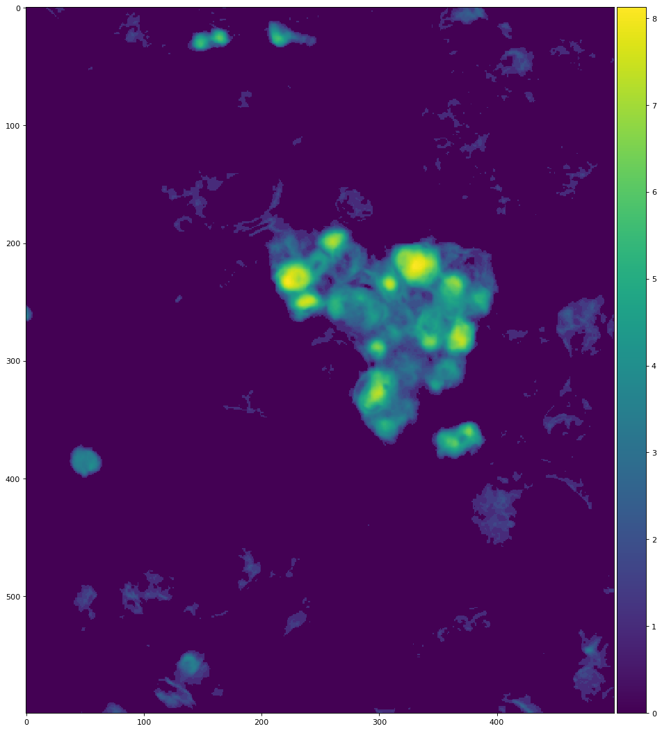
This is a different view of the tissue. These pixels are a signal representation of dectected abnormal protein aggregates.

Sample source code part 10

import numpy as np
overlayImage = np.dstack((EMimage+vectors,EMimage,EMimage))

figure(figsize=(12, 18), dpi=80)
io.imshow(overlayImage)
plt.show()

This overlay colorizes the abnormal protin cluster

Sample source code part 11

from skimage.filters import gaussian

glycogen = io.imread(alzdata['Glycogen'][-1])[1300:1900,2000:2500]
mitochondria = io.imread(alzdata['Mitochondria'][-1])[1300:1900,2000:2500]
vesicles = io.imread(alzdata['Vesicles'][-1])[1300:1900,2000:2500]

# normalize the signal from various structures to a 0-1 range with disntinctive contrast
glycogen = 100*glycogen**.8
mitochondria = gaussian(80*mitochondria**.5,6)**1.1
glycogen = glycogen/mitochondria.max()
mitochondria = mitochondria/mitochondria.max()

vesicles = vesicles*(mitochondria.max()/vesicles.max())
vesicles = vesicles**2
vesicles = vesicles/vesicles.max()
vesicles[vesicles>1] = 1

vectors = vectors/vectors.max()

figure(figsize=(12, 18), dpi=80)
io.imshow(np.hstack((glycogen,mitochondria,vesicles, vectors)))
plt.show()

There are many different structures that these images contain. On the far-left is signal for glycogen, a molecular sugar complex that astrocyte's use to transport energy to neurons and synapses. These samples are particularily enriched with glycogen, which could indicate a metabolic dishomeostasis.

The center-left is mitochondria, which are import both for energy production and synaptic transmission.

The center-right is signal predicting synaptic vesicles, which contain the neurotransmitter that neurons use to communicate with one another.

The far-right is the same protein aggregate signal from above

Sample source code part 12

from distinctipy import distinctipy
import random

# set a seed so the same colors are chosen
random.seed(1); cols = distinctipy.get_colors(4,exclude_colors=[(0.5,.5,0.5),(0,0,0),(1,1,1)],pastel_factor = .3)

visual = np.dstack([EMimage]*3)/255
EMonly = visual.copy()
for i, prob in zip(range(4), [vectors, glycogen, mitochondria, vesicles]):
prob = np.dstack([prob]*3)
for c in range(prob.shape[2]):
prob[:,:,c] = prob[:,:,c]*cols[i][c]
visual = visual+prob
figure(figsize=(18, 24), dpi=80)
io.imshow(np.hstack((EMonly, .4*np.ones((visual.shape[0],50,3)), visual)))
plt.show()

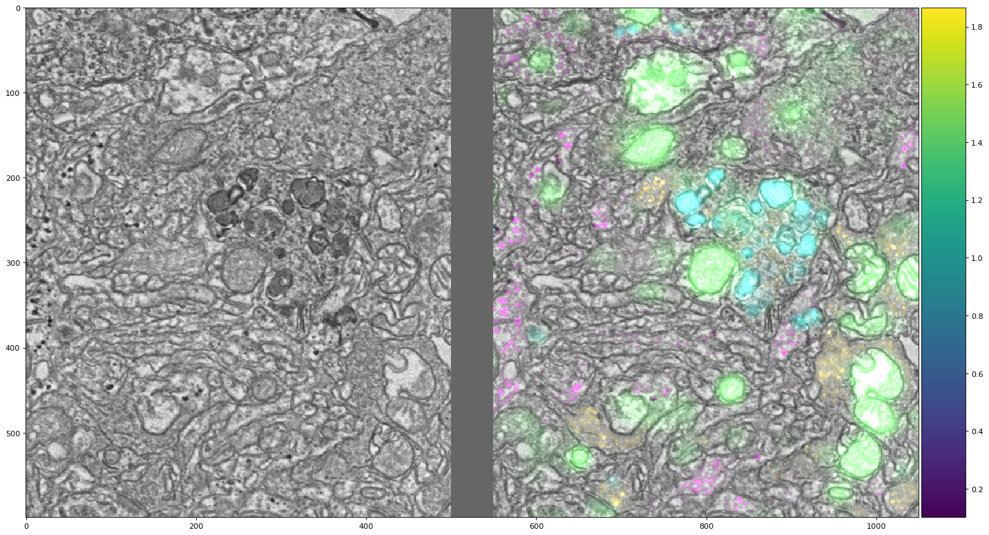
This color composite highlights the variety of structures in this image. Glycogen (magenta), synaptic vesicles (yellow), mitochondria (green), and protein aggregates (teal) organize themsel

For developers

Launch an interactive demo
*This button will launch an interactive Jupyter session that will introduce you to the appearance of biopsy tissue, pathological structures-of-interest, and 3D image data.